In-memory LPG primer

General background on holding a graph in RAM, querying it with a handful of small functions, and the measurements that explain why the structure is shaped the way it is. It describes the model rather than any one program, and the Go is illustrative: something to copy and adapt, not a package to import.

---

Summary

• A Labeled Property Graph (LPG) is nodes and directed, typed edges where nodes and edges alike carry a free-form property map. Property maps on the edge distinguish the model (§1).
• Hold it in memory as typed structs + a few maps: nodes/edges by id, an adjacency index (out/in), and a label index (byLabel). Build the indexes at insert time; reads stay cheap (§2).
• Those indexes earn their cost. On a 100k-node / 600k-edge graph, indexed neighbor lookup measured ~21,000× faster than a flat-slice scan, and a selective label lookup ~1,500× faster. A non-selective label lookup, one that matches a large share of the nodes, measured only ~1.35× faster, because materializing 20k results dominates. The index helps in proportion to how much it lets you skip (§4).
• You can start without a query language. A fixed set of typed, bounded verbs covers most real questions: lookup, one-hop, k-hop BFS (breadth-first search), pattern+filter, and path existence. Because there is no query text, there is no parser to maintain and no query string for a caller to smuggle anything into, and every traversal takes a depth limit as an argument, so none of them can be called unbounded (§3). Move to a real query engine only when open-ended querying is a requirement (§5).

---

1. What an LPG is (the pragmatic version)

A Labeled Property Graph is just two kinds of things:

• Nodes — entities. Each node has one or more labels (its type(s), e.g. Person, Company) and a map of properties (arbitrary key→value, e.g. name: "Alice", founded: 2001).
• Edges (a.k.a. relationships) — connections. Each edge is directed (from → to), has exactly one type (e.g. WORKS_AT, KNOWS), and, the defining feature, also carries its own map of properties (e.g. since: 2021, role: "eng").

The worked example throughout is people, companies, and who knows / works-at / founded whom; substitute your own labels, because nothing in the model depends on that choice.

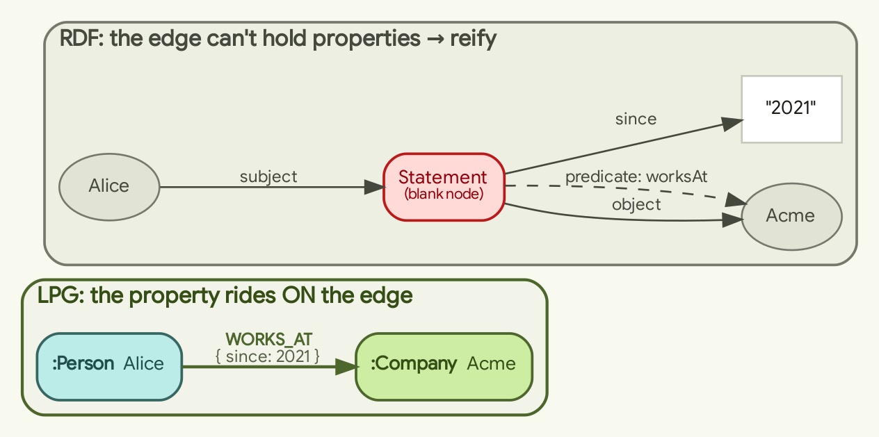
Edges carrying their own properties are the reason the LPG exists as a distinct model. In RDF the graph is a set of subject–predicate–object triples whose parts are named by globally unique identifiers (IRIs), and the edge (the predicate) cannot natively hold properties. To say “Alice worked at Acme since 2021” you must either use reification, which means turning the statement itself into an extra node so that facts about the statement have somewhere to attach, or named graphs, which means putting the triple in its own separately labeled subgraph and attaching the extra facts to that. In an LPG the edge is an object in its own right, with the same standing as a node. It has its own identity and its own property map: (:Person)-[:WORKS_AT {since:2021, role:"eng"}]->(:Company). The extra detail lives on the relationship itself. That is why an LPG tends to match how people already describe their data, and why information about where a fact came from and how much to trust it (“who said this, when, how confident”) sits on the edge.

Standards grounding:

• GQL — ISO/IEC 39075:2024 — the first standalone ISO graph query language (“first new ISO database language since SQL”), declarative, for property graphs.
• SQL/PGQ — ISO/IEC 9075-16:2023 — property-graph pattern matching inside a SQL SELECT.
• openCypher / Cypher — the most widely used LPG query language, a standard by adoption rather than by publication (Neo4j lineage), and a key inspiration for GQL; what the examples below map to.

Everything below is how you realize that model in memory, and the small set of operations you run on it.

---

2. In-memory structure

2.1 The two element types as typed structs

type ID string

// Node: an entity with labels (types) and a free-form property bag.
type Node struct {
  ID     ID
  Labels []string       // e.g. ["Person"]  (a node may carry several)
  Props  map[string]any // e.g. {"name": "Alice", "born": 1990}
}

// Edge: a directed, typed relationship that ALSO carries properties.
type Edge struct {
  ID    ID
  Type  string         // exactly one type, e.g. "WORKS_AT"
  From  ID             // source node id
  To    ID             // target node id
  Props map[string]any // e.g. {"since": 2021, "role": "eng"}
}

map[string]any is the pragmatic choice for the property bag. It mirrors the fact that an LPG does not require a schema: two Person nodes may carry different property keys, and nothing rejects them. (If your properties are known and fixed, a typed struct per label is faster and safer, but map[string]any is what keeps the container general.)

2.2 The container — and why it needs indexes

The naive container is nodes plus a flat edges slice. It holds a graph well enough and traverses one badly: “who does Alice work for?” would scan every edge: O(E) per hop, meaning the cost grows with the total number of edges in the graph. Real in-memory graphs keep a few indexes so that the operations you run most often stay cheap:

type Graph struct {
  nodes map[ID]*Node // id -> node   (O(1) lookup by id)
  edges map[ID]*Edge // id -> edge

  // Adjacency indexes: node -> the edge ids touching it.
  out map[ID][]ID // node -> outgoing edge ids  (O(deg) neighbor scan)
  in  map[ID][]ID // node -> incoming edge ids

  // Label index: label -> node ids carrying it.
  byLabel map[string][]ID // "Person" -> [ids]  (O(1) to get the label's set)
  // (optional) property index: e.g. map[string]map[any][]ID for exact-match
  // lookups on a hot property — add only when a scan proves too slow.
}

func NewGraph() *Graph {
  return &Graph{
    nodes: map[ID]*Node{}, edges: map[ID]*Edge{},
    out: map[ID][]ID{}, in: map[ID][]ID{}, byLabel: map[string][]ID{},
  }
}

Maintain the indexes at insert time so reads stay cheap:

func (g *Graph) AddNode(n *Node) {
  g.nodes[n.ID] = n
  for _, l := range n.Labels {
    g.byLabel[l] = append(g.byLabel[l], n.ID)
  }
}

func (g *Graph) AddEdge(e *Edge) {
  g.edges[e.ID] = e
  g.out[e.From] = append(g.out[e.From], e.ID) // forward adjacency
  g.in[e.To] = append(g.in[e.To], e.ID)       // reverse adjacency
}

Why these two indexes are worth their cost:

• Adjacency (out/in) narrows “neighbors of v” to the edges attached to v, because those are the only ones you need to look at. Indexing each direction lets you traverse forward and backward without re-scanning.
• Label index (byLabel) turns “all Person nodes” from an O(N) scan of every node into an O(1) map hit (one lookup whose cost does not grow with the graph) that returns the ready-made id list.

A couple of maps built at insert time make traversal and label scans cheap on read. §4 shows what that is worth in nanoseconds.

2.3 Complexity at a glance

Operation	Naive (flat slices)	With indexes
Lookup node by id	O(N)	O(1)
All nodes with label L	O(N)	O(|L|) (just the matches)
Out-neighbors of v by type	O(E)	O(deg(v))
k-hop bounded BFS	O(k·E)	O(visited + edges touched)
Bounded path existence	O(k·E)	O(visited + edges touched)

The indexed column never scans the whole graph to answer a local question.

2.4 Building one (usage)

g := NewGraph()
g.AddNode(&Node{ID: "p:alice", Labels: []string{"Person"}, Props: map[string]any{"name": "Alice"}})
g.AddNode(&Node{ID: "p:bob",   Labels: []string{"Person"}, Props: map[string]any{"name": "Bob"}})
g.AddNode(&Node{ID: "c:acme",  Labels: []string{"Company"}, Props: map[string]any{"industry": "tech"}})

g.AddEdge(&Edge{ID: "e1", Type: "WORKS_AT", From: "p:alice", To: "c:acme", Props: map[string]any{"since": 2021}})
g.AddEdge(&Edge{ID: "e2", Type: "KNOWS",    From: "p:alice", To: "p:bob",  Props: map[string]any{"since": 2019}})
g.AddEdge(&Edge{ID: "e3", Type: "FOUNDED",  From: "p:bob",   To: "c:acme"})

---

3. Querying the in-memory LPG (the operations you run)

Each operation is a small typed function, shown next to the Cypher it corresponds to. This is the fixed-verb style (option (a) in §5): a closed set of named operations instead of a query language.

3.1 Lookup by id / by label

func (g *Graph) Node(id ID) (*Node, bool) { n, ok := g.nodes[id]; return n, ok }

func (g *Graph) NodesByLabel(label string) []*Node {
  ids := g.byLabel[label]
  out := make([]*Node, 0, len(ids))
  for _, id := range ids {
    out = append(out, g.nodes[id])
  }
  return out
}

MATCH (n) WHERE n.id = $id RETURN n        -- Node(id)
MATCH (n:Person) RETURN n                  -- NodesByLabel("Person")

3.2 Neighbors / one-hop traversal by edge type

// OutNeighbors: nodes reachable from `id` via ONE edge of type `etype`.
func (g *Graph) OutNeighbors(id ID, etype string) []*Node {
  var res []*Node
  for _, eid := range g.out[id] { // only edges touching `id`
    if e := g.edges[eid]; e.Type == etype {
      if n, ok := g.nodes[e.To]; ok {
        res = append(res, n)
      }
    }
  }
  return res
}

MATCH (a)-[:WORKS_AT]->(b) WHERE a.id = $id RETURN b

Swap g.out for g.in (and e.From) to walk relationships backward (MATCH (a)<-[:WORKS_AT]-(b)).

3.3 k-hop / bounded neighborhood (BFS with a depth cap)

// NeighborhoodBFS: all nodes within `maxDepth` out-hops of `start`,
// returned as id -> distance. The `dist` map doubles as the visited set.
func (g *Graph) NeighborhoodBFS(start ID, maxDepth int) map[ID]int {
  dist := map[ID]int{start: 0}
  queue := []ID{start}
  for len(queue) > 0 {
    cur := queue[0]
    queue = queue[1:]
    d := dist[cur]
    if d == maxDepth { // depth bound: stop expanding here
      continue
    }
    for _, eid := range g.out[cur] {
      nxt := g.edges[eid].To
      if _, seen := dist[nxt]; !seen { // cycle/re-visit guard
        dist[nxt] = d + 1
        queue = append(queue, nxt)
      }
    }
  }
  return dist
}

MATCH (a)-[*1..3]->(b) WHERE a.id = $id RETURN DISTINCT b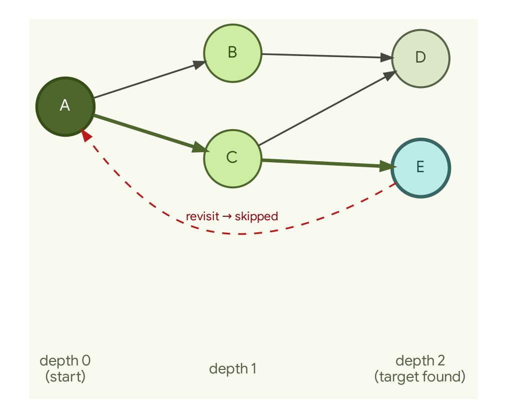

Why bounding matters: a graph can contain cycles and can be densely connected, so an unbounded walk can revisit nodes forever, fan out across the whole graph, or both. Two guards are required: (1) a visited set (here, dist itself) so that cycles terminate, and (2) a depth cap (maxDepth) so that cost stays predictable. Without both, “expand from a node” is an easy way to hang the process or exhaust memory on a graph that looked small. This is also the reason a query surface should make callers pass a bound rather than defaulting to one.

3.4 Pattern match + filter

“Find people who work at a company in a given industry” is a two-element pattern with a property predicate on the far node:

// PeopleInIndustry: Person nodes with a WORKS_AT edge to a Company
// whose `industry` property equals `want`.
func (g *Graph) PeopleInIndustry(want string) []*Node {
  var res []*Node
  for _, pid := range g.byLabel["Person"] { // label index: start narrow
    for _, eid := range g.out[pid] {
      e := g.edges[eid]
      if e.Type != "WORKS_AT" {
        continue
      }
      if c := g.nodes[e.To]; c != nil && c.Props["industry"] == want {
        res = append(res, g.nodes[pid])
        break // one match is enough; avoid dupes
      }
    }
  }
  return res
}

MATCH (p:Person)-[:WORKS_AT]->(c:Company)
WHERE c.industry = $want
RETURN DISTINCT p

The shape mirrors the Cypher: start from the cheapest anchor, meaning the smallest starting set an index can hand you (here the label index), walk the typed edge, then apply the WHERE on properties. A database engine’s query planner picks that starting set for you; here you pick it yourself, taking Person, or Company if there are fewer of them.

3.5 Bounded path existence between two nodes

// PathExists: is `dst` reachable from `src` within `maxDepth` out-hops?
func (g *Graph) PathExists(src, dst ID, maxDepth int) bool {
  if src == dst {
    return true
  }
  visited := map[ID]bool{src: true}
  type item struct {
    id    ID
    depth int
  }
  queue := []item{{src, 0}}
  for len(queue) > 0 {
    cur := queue[0]
    queue = queue[1:]
    if cur.depth == maxDepth {
      continue
    }
    for _, eid := range g.out[cur.id] {
      nxt := g.edges[eid].To
      if nxt == dst {
        return true
      }
      if !visited[nxt] {
        visited[nxt] = true
        queue = append(queue, item{nxt, cur.depth + 1})
      }
    }
  }
  return false
}

MATCH (a), (b) WHERE a.id = $src AND b.id = $dst
RETURN EXISTS { MATCH (a)-[*..4]->(b) }

Same BFS skeleton as §3.3, with an early return on hitting dst and the same two guards.

3.6 Going a little further: shortest path and aggregation

Both of the operations below are the same primitives (adjacency walk + a bound), carrying a bit more state.

Shortest path (by hop count), with reconstruction. BFS already visits nodes in increasing distance, so the first arrival at dst is via a shortest path. Carry a predecessor map and walk it backward to rebuild the route:

// ShortestPath: node sequence [src..dst] via fewest hops, bounded by maxDepth.
// Returns nil if dst is unreachable within the bound.
func (g *Graph) ShortestPath(src, dst ID, maxDepth int) []ID {
  if src == dst {
    return []ID{src}
  }
  prev := map[ID]ID{src: ""} // child -> parent; doubles as visited set
  depth := map[ID]int{src: 0}
  queue := []ID{src}
  for len(queue) > 0 {
    cur := queue[0]
    queue = queue[1:]
    if depth[cur] == maxDepth {
      continue
    }
    for _, eid := range g.out[cur] {
      nxt := g.edges[eid].To
      if _, seen := prev[nxt]; seen {
        continue
      }
      prev[nxt] = cur
      depth[nxt] = depth[cur] + 1
      if nxt == dst { // reconstruct src..dst
        path := []ID{dst}
        for at := cur; at != ""; at = prev[at] {
          path = append(path, at)
        }
        for i, j := 0, len(path)-1; i < j; i, j = i+1, j-1 {
          path[i], path[j] = path[j], path[i] // reverse in place
        }
        return path
      }
      queue = append(queue, nxt)
    }
  }
  return nil
}

MATCH p = shortestPath((a)-[*..4]->(b))
WHERE a.id = $src AND b.id = $dst
RETURN p

(For weighted edges, say a cost property, swap BFS for Dijkstra; the shape is the same, a priority queue instead of a first-in, first-out (FIFO) queue.)

Aggregation. Counting/grouping over a node’s edges is just a walk into a map:

// OutDegreeByType: count of outgoing edges of `id`, grouped by edge type.
func (g *Graph) OutDegreeByType(id ID) map[string]int {
  deg := map[string]int{}
  for _, eid := range g.out[id] {
    deg[g.edges[eid].Type]++
  }
  return deg
}

MATCH (a)-[r]->() WHERE a.id = $id
RETURN type(r) AS type, count(*) AS n

---

4. What the indexes are worth (measured)

Every performance claim on this page is measured rather than estimated. The complexity claims in §2 are easy to assert; here is what they cost in nanoseconds. All numbers come from Go benchmarks (go test -bench . -benchmem) on a synthetic graph built with a fixed-seed pseudo-random number generator, so every run builds the same graph and the results are reproducible. The harness is in the appendix (§7) and the machine is in the environment block below.

Benchmark environment. goos: linux, goarch: amd64, Intel Xeon @ 2.80GHz, 2 CPUs, Go toolchain default settings. Graph: 100,000 nodes, 600,000 edges, 5 labels, 3 edge types. “Naive” = the same query implemented over a flat []*Edge / []*Node slice with no adjacency or label index.

Benchmark	Indexed	Naive	Speedup
Out-neighbors of one node, by type	385.6 ns/op	8,078,786 ns/op	~21,000×
Label lookup, selective (10 of 100k match)	319.6 ns/op	484,456 ns/op	~1,500×
Label lookup, non-selective (~20k of 100k match)	1,176,413 ns/op	1,584,779 ns/op	~1.35×

Reproducibility note. The selective row above (319.6 ns/op, ~1,500×) is not reproducible from the harness as printed in §7. That listing builds only the evenly distributed labels L0–L4 and benchmarks NodesByLabel("L0"), which is the non-selective row. §7’s closing paragraph describes the rare-label setup this selective row needs, but the code that produced it is not shown on this page, so running the printed harness alone will not regenerate this one row.

1. Adjacency indexing is a requirement at scale. One neighbor lookup over 600k edges went from ~8 ms (a full scan) to ~386 ns, about four orders of magnitude. Any traversal does this per hop, so the gap compounds fast.

2. A label index helps in proportion to how much it lets you skip. For a selective label (10 matching nodes) it is ~1,500× faster, because the naive version still walks all 100k nodes while the index jumps straight to the 10. But for a non-selective label (~20k matches) the speedup collapses to ~1.35×: both versions must now touch and materialize ~20k results, and that work, not the lookup, dominates. An index accelerates the search, never the size of the answer. If your query returns a big fraction of the graph, no index saves you; the fix is to return less: filter, paginate, or push the predicate down, which means applying the filter at the source instead of over the assembled results.

An index therefore answers some questions cheaply and leaves others as expensive as they were, which is why the fixed-verb API in §3 makes callers pass bounds: the cheapest result set is the one you never materialize.

---

5. Two ways to expose all this — and why fixed verbs are the light start

• (a) A fixed set of typed query functions — exactly §3: Node, NodesByLabel, OutNeighbors, NeighborhoodBFS, PeopleInIndustry, PathExists, ShortestPath, OutDegreeByType. Pragmatic, safe, and free of dependencies. There is no query string to parse, so there is no query text in which a caller could hide an instruction you did not intend to run; every traversal takes its bound as a required argument (the caller passes maxDepth), so an unbounded walk is not expressible; and the set of operations is small enough to review in one sitting. This is the lightweight starting point.
• (b) Parse a query language (Cypher / GQL / SQL-PGQ) — accept a query string, tokenize → parse → plan → execute over the same in-memory structures. Far more flexible (arbitrary patterns, aggregation, projection), but it brings in a parser and a planner; it means accepting query text you did not write, which has to be treated as untrusted; and it hands the bounding problem back to you: you must cap traversal depth and result size yourself, or a single query can walk the whole graph (see §4). That is the right move once ad-hoc querying becomes a requirement.

Rule of thumb: start with (a): a handful of typed, bounded verbs covering the 90% of questions asked. Graduate to (b), or better to an engine that already implements a standard language (§6), only when open-ended querying is a real requirement.

---

6. When you outgrow in-memory

The in-memory LPG is ideal while the graph fits in RAM, is rebuilt from a source of truth (so you don’t need durability), and has one writer. You graduate when any of those breaks:

• Doesn’t fit / needs persistence / concurrent writers / transactions → an embedded engine: e.g. DuckDB + the DuckPGQ extension, which gives you SQL/PGQ (ISO/IEC 9075-16:2023) over local data, a real standard query language in-process.
• Needs scale-out, an operational store, or a managed service → a server: Spanner Graph (ISO-GQL) or Neo4j (Cypher/GQL), etc.

The pragmatic progression is therefore in-memory typed verbs → embedded engine (SQL/PGQ / Cypher) → remote managed graph (GQL). You add a query language, and then a server, when the workload demands it.

Choosing between the engines above is its own exercise, and it is worth doing before you commit: compare the query language each one speaks and which standard it belongs to, the license, how actively the project is maintained, and whether it runs in your process or as a server you have to operate. Consult each project’s own documentation for the current answers rather than a snapshot in a page like this one.

---

7. Appendix — the benchmark harness (reproduce the §4 numbers)

A deterministic linear-congruential generator (LCG) builds the graph so every run is identical; each benchmark compares the indexed method against a naive flat-slice equivalent.

// graph_test.go — run with: go test -bench . -benchmem
package lpgbench

import (
  "fmt"
  "testing"
)

// deterministic linear-congruential generator (reproducible graphs)
type lcg struct{ s uint64 }

func (r *lcg) next() uint64 { r.s = r.s*6364136223846793005 + 1442695040888963407; return r.s }
func (r *lcg) intn(n int) int { return int(r.next() >> 33 % uint64(n)) }

const (
  N      = 100_000
  M      = 600_000
  nLabel = 5
  nType  = 3
)

func buildGraph() *Graph {
  g := NewGraph()
  r := &lcg{s: 12345}
  for i := 0; i < N; i++ {
    id := ID(fmt.Sprintf("n%d", i))
    g.AddNode(&Node{ID: id, Labels: []string{fmt.Sprintf("L%d", i%nLabel)}})
  }
  for i := 0; i < M; i++ {
    from := ID(fmt.Sprintf("n%d", r.intn(N)))
    to := ID(fmt.Sprintf("n%d", r.intn(N)))
    g.AddEdge(&Edge{ID: ID(fmt.Sprintf("e%d", i)), Type: fmt.Sprintf("T%d", i%nType), From: from, To: to})
  }
  return g
}

func BenchmarkOutNeighborsIndexed(b *testing.B) {
  g := buildGraph()
  b.ResetTimer()
  for i := 0; i < b.N; i++ {
    _ = g.OutNeighbors("n42", "T0")
  }
}

func BenchmarkOutNeighborsNaive(b *testing.B) {
  g := buildGraph()
  b.ResetTimer()
  for i := 0; i < b.N; i++ {
    _ = g.OutNeighborsNaive("n42", "T0")
  }
}

func BenchmarkNodesByLabelIndexed(b *testing.B) {
  g := buildGraph()
  b.ResetTimer()
  for i := 0; i < b.N; i++ {
    _ = g.NodesByLabel("L0")
  }
}

func BenchmarkNodesByLabelNaive(b *testing.B) {
  g := buildGraph()
  b.ResetTimer()
  for i := 0; i < b.N; i++ {
    _ = g.NodesByLabelNaive("L0")
  }
}

The naive baselines (in the same package) scan the flat slices the indexes exist to avoid:

// naive baselines keep a flat []*Edge / []*Node and scan them.
func (g *Graph) OutNeighborsNaive(id ID, etype string) []*Node {
  var res []*Node
  for _, e := range g.edgeList { // every edge in the graph
    if e.From == id && e.Type == etype {
      if n, ok := g.nodes[e.To]; ok {
        res = append(res, n)
      }
    }
  }
  return res
}

func (g *Graph) NodesByLabelNaive(label string) []*Node {
  var res []*Node
  for _, n := range g.nodeList { // every node in the graph
    for _, l := range n.Labels {
      if l == label {
        res = append(res, n)
        break
      }
    }
  }
  return res
}

Note: these snippets are illustrative, not a complete program. They are deliberately elided for readability rather than a single package you can build. In particular the naive baselines above iterate g.edgeList and g.nodeList — flat-slice fields that the Graph struct in §2.2 does not declare (it keeps only the maps nodes, edges, out, in, byLabel) — so this listing will not go build as printed. Read it as a faithful sketch of the approach, not code to paste and run.

The selectivity result (§4, row 2 vs row 3) comes from adding a rare label RARE to just 10 of the 100k nodes and benchmarking NodesByLabel("RARE") (10 matches, ~1,500×) against NodesByLabel("L0") (~20k matches, ~1.35×): same code, different selectivity, opposite conclusion.

---

Sources

• GQL — ISO/IEC 39075:2024 (iso.org/standard/76120.html; en.wikipedia.org/wiki/Graph_Query_Language). SQL/PGQ: ISO/IEC 9075-16:2023.
• openCypher — opencypher.org. Cypher — neo4j.com/docs/cypher-manual/current.
• LPG data model vs RDF triples (edges carrying their own properties) — RDF 1.1 Concepts, w3.org/TR/rdf11-concepts/, which defines the triple model and the reification and named-graph workarounds described in §1.
• Embedded and remote engines — DuckDB + the DuckPGQ extension, Spanner Graph, and Neo4j; see each project’s own documentation for its current query-language support, license, and maintenance status.
• Performance numbers (§4) — measured by the author with the harness in §7; goos linux, goarch amd64, Intel Xeon @ 2.80GHz, 2 CPUs; 100k nodes / 600k edges.
• Figures — authored in Graphviz DOT and stored next to this page as DOT source plus a lossless WebP render (dot→PNG→cwebp); sources, render command, and the font/theme note live in assets/README.md. Font: Google Sans Flex (fonts.google.com). Palette: Material light theme (owner-supplied).